QPSK: Over-the-Air With Pluto Radios

Introduction

Many of previous QPSK Simulink exercises assumed perfect synchronization, perfect timing synchronization, or perfect phase synchronization, or both. It is now time to explore how it is in practice--neither carrier phase nor timing is known to the detector and must be estimated. Simultaneous carrier phase and symbol timing synchronization is an example of a joint estimator: more than one unknown parameter is estimated. This is accomplished using two PLLs, one for timing synchronization (the inner loop) and one for carrier phase synchronization (the outer loop). The issue of carrier phase ambiguity is still with us, so differential encoding is also used here.

In this exercise, you will design a joint carrier phase and symbol timing timing synchronizer for QPSK based on two PLLs. There are three sample rates in play in this design, so you must be careful in assigning sample times to the Simulink blocks.

This project is based on a Software Defined Radio (SDR) known as the Pluto Radio. The Pluto Radio was developed by Analog Devices and is supported in a big way by the MathWorks. The Pluto Radio is an external radio that connects to your computer via a USB cable.

This exercise is divided into two parts. In the first part, you will design and debug your system to operate with samples captured from a Pluto radio output. In the second part, you will replace the input to your Simulink design with a Simulink block that interfaces with the Pluto Radio. A signal is transmitted from one Pluto Radio, and received by a second Pluto radio connected to your computer. The Pluto radio produces I/Q samples (organized into complex-valued numbers) that are processed by your Simulink design.

Textbook References

M-ary QAM: Section 5.3, discrete-time realizations: Section 5.3.2, partial response pulse shapes: Section A.2, discrete-time PLL: Section C.2, carrier phase synchronization for QPSK: Section 7.2, differential encoding for phase ambiguity resolution for QPSK: Section 7.7.2, general discussion of timing synchronization: Section 8.1, discrete-time techniques for symbol timing synchronization for binary PAM: Section 8.4, discrete-time techniques for symbol timing synchronization for MQAM: Section 8.5.

Specifications

	Transmitter Specifications carrier frequency: 425 MHz data rate: 40 ksymbols/s (80 kbits/s) pulse shape: SRRC (50% excess bandwidth, span = 12 symbols) phase ambiguity resolution: differential encoding bits phase shift ------------------ 00 0 deg 01 90 deg 10 -90 deg 11 180 deg packet format: PRE = 1 1 ... 1 (64 bits -- all ones) DATA = 5404 bits
	Demodulator Specifications input: Part 1: the data vector contained in the file TestInput.mat Part 2: the output of the Pluto Radio block average energy: you define this symbol clock offset: unknown!! carrier phase unknown!!

Pluto Radio Overview

A (very) simplified block diagram the Pluto Radio as a radio receiver is shown below.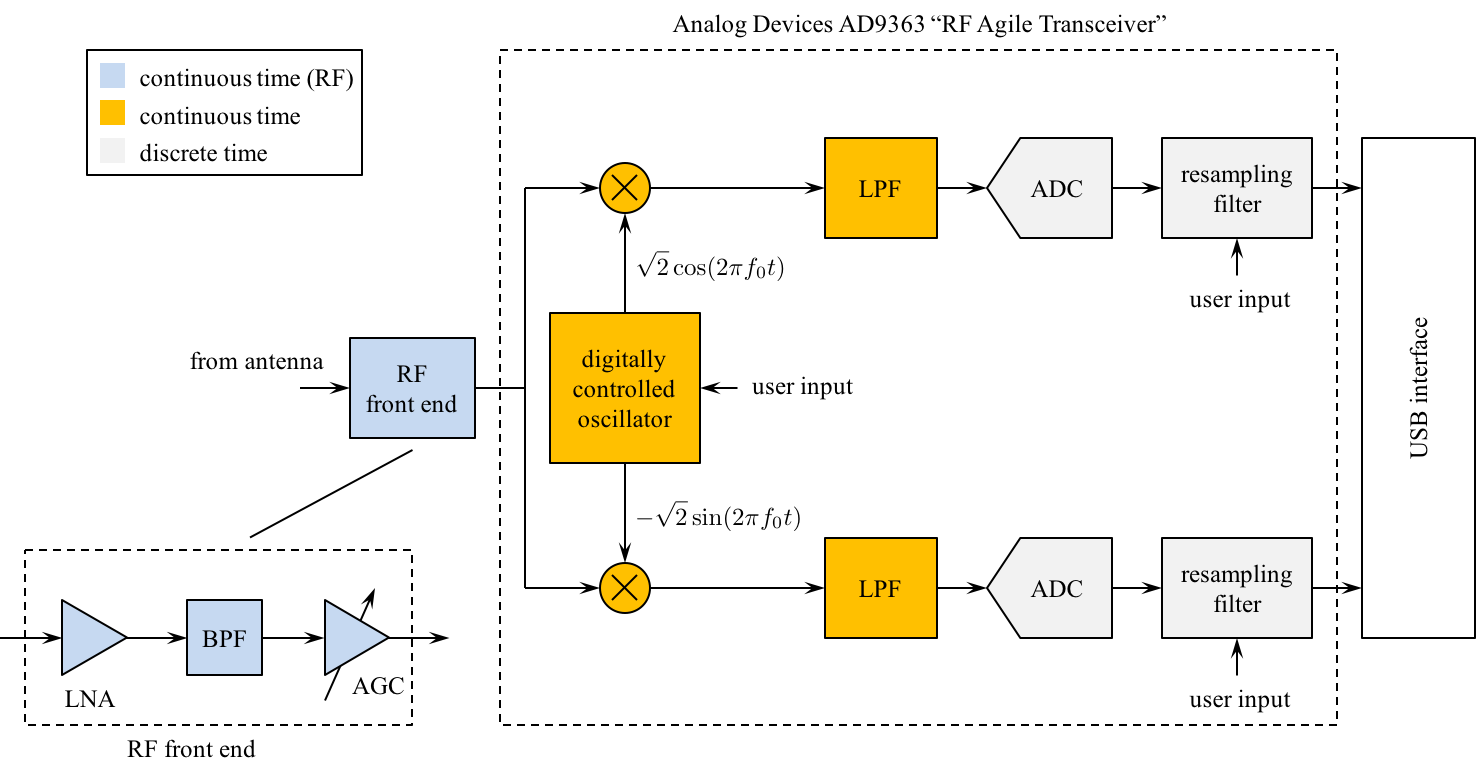

• The Pluto Radio comprises a software configurable RF Front End, I/Q Mixer to perform quadrature down-conversion, and a pair of analog-to-digital converters (ADCs) operating on the filtered quadrature downconverter outputs.


• The center frequency used by the quadrature downconverter is specified by the user.


• The desired sample rate for the I/Q samples is obtained from the (high) sample rate signal using resampling filters. (See Section 9.3 of the text.) The desired sample rate is specified by the user --- one usually selects an integer multiple of the symbol rate.


• The I/Q samples are transferred to your computer via a USB interface and appear in Matlab and Simulink as a vector of complex-valued variables: the real part is the inphase component (I) and the imaginary part is the quadrature component (Q).

Part 1

Design the Detector

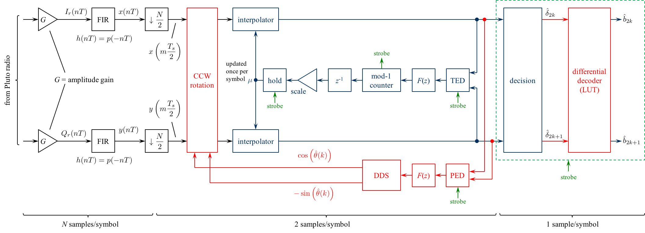
Design the detector, shown below, using blocks from the Simulink, DSP System, and Communications System Toolboxes.

Design Notes

1. To separate the I/Q components from the complex-valued input, use the block
   
   Simulink -> Math Operations -> Complex to Real-Imag


2. The gain blocks is used to scale the Pluto Radio output to the desired average energy. This needs to be done only once because the Pluto Radio RF front end is equipped with an Automatic Gain Control (AGC) circuit. [See Section 9.5 (pp. 546 - 551) of the text.] This scaling is important because the TED and PED gains (both Kp) are proportional to the input signal level. Hints for getting the scaling right.
   
   It cannot be overemphasized how important this step is. Also note that the scale factor that needs to be applied depends on the version of Simulink used. It is impossible here to include test files for all the different versions. Consequently, when you get to Part 2 where data from the Pluto Radio is used, you will need to recheck the scaling used. Perform this "recheck" using data from the Pluto Radio.


3. The number of samples/symbol is determined by the sample rate you specify. My experience with the computers in the lab is that a good design can operate at an input sample rate of 160 ksamples/s. This produces N = 160 ksamples/s / 40 ksymbols/s = 4 samples/symbol.


4. Use the early-late TED. Because the early-late TEDs operate at 2 samples/symbol, the matched filter output must be downsampled to 2 samples/symbol.


5. The carrier phase synchronization loop is the outer loop shown in red.


1. In the two previous two Simulink exercises devoted to carrier phase synchronization for QPSK (Carrier Phase Synchronization for QPSK Using the Unique Word and Carrier Phase Synchronization for QPSK Using Differential Encoding/Decoding), perfect timing synchronization was assumed and this assumption allowed the carrier phase PLLs to operate at one sample per symbol.


2. In contrast, the matched filter outputs here are at 2 samples/symbol. Consequently, the CCW rotation block operates at 2 samples/symbol.


3. The PED operates at 2 samples/symbols, but only updates at 1 sample/symbol. This is why the PED needs to strobe input. When the strobe is asserted, the PED output follows the formula (7.26) on page 343. When the strobe is not asserted, the PED output is zero. (For those of you familiar with multirate discrete-time processing, this is like an upsample-by-two operation.)


4. The loop filter and DDS operate at 2 samples/symbol. (In the context of multirate processing, the PED does the upsample-by-two and the loop filter is the "interpolating filter" to smooth out the inserted zeros.)


5. Design the loop filter to create a second order PLL with a closed-loop bandwidth of 2% of the symbol rate and a damping factor of 0.7071. You may need to increase the closed-loop bandwidth depending on the carrier frequency offset you experience. Each radio produces its own frequency offset.


6. The symbol timing PLL is the inner loop shown in blue. Except for the CCW rotation block, the symbol timing PLL is identical to the one you designed for the Symbol Timing Synchronization for QPSK Simulink Exercise.


1. Use a Farrow interpolator. You can use either the piecewise-parabolic version (see Figure 8.4.17) or the cubic version (see Figure 8.4.18).


2. For interpolation control, use the decrementing modulo-1 counter described in Section 8.4.3. Use the underflow condition in the decrementing modulo-1 counter to assert the strobe. The strobe is used as an enable signal for the TED, PED, decision, and fractional interpolation interval update.


3. You need to create an "enabled" version of the early-late TED. When the strobe is asserted, the TED output is given by equation (8.34). When the strobe is not asserted, the TED output is zero.



4. For the fractional interval (mu) update, use an "enabled hold" block. The "enabled hold" block outputs the previous value when the strobe is not asserted, or passes the input to the output when the strobe is asserted. This block is needed because the fractional interval is updated by the mod-1 counter only once per symbol, but the interpolator operates at 2 samples/symbol. The hold operation ensures that the interpolator is using the proper value for the fractional interval.
   
   Simulink provides a skeletal enabled subsystem:
   
      Simulink -> Ports & Subsystems -> Enabled Subsystem
   
   The default enabled subsystem is shown below
   
   
   
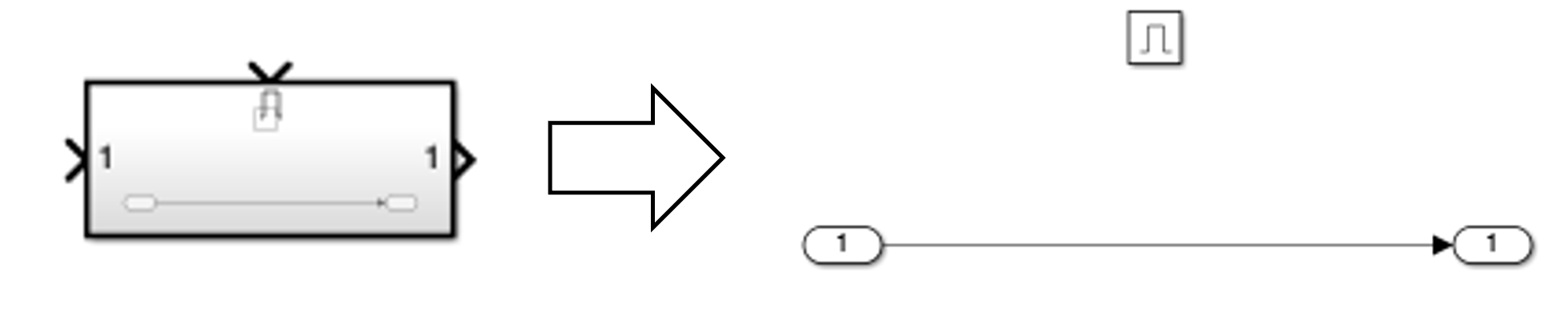
   The subsystem consists of a simple wire with the enable icon above it. This means the wire is only active when the enable signal (strobe in this case) is asserted. When the enable signal (strobe in this case) not asserted, nothing happens and the output holds its value.


5. Design the loop filter to create a second order PLL with a closed-loop bandwidth of 1% of the symbol rate and a damping factor of 0.7071.


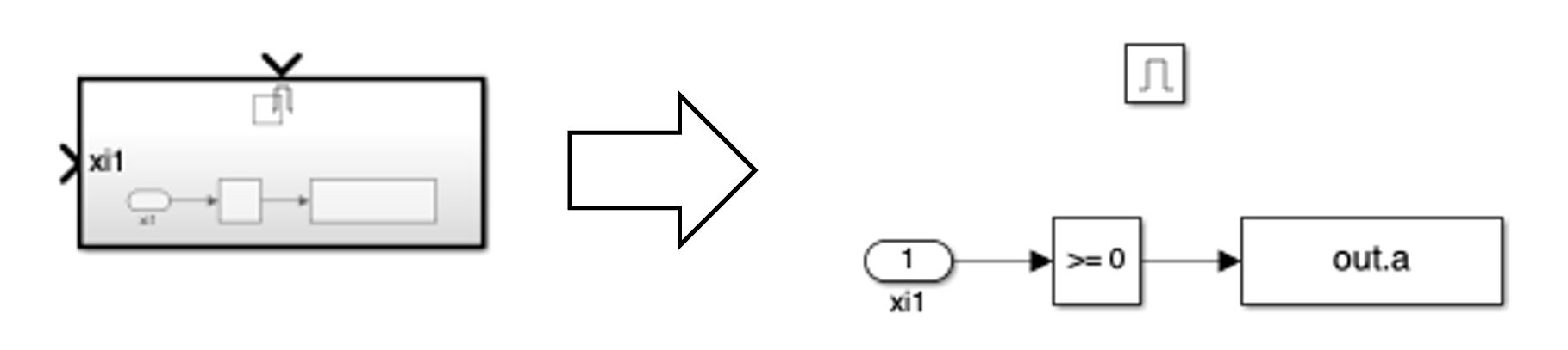
7. The decision subsystem is also enabled. This is because decisions should be made on every other interpolator output on average. The strobe indicates which interpolator outputs represent the desired signal space projections. An example of the enabled decision subsystem for binary PAM is shown below.
   
   
   
   

Exercise

1. Design the detector shown above using blocks from the Simulink, DSP System, and Communications System Toolboxes.


2. For the detector input, use the block
   
   DSP System Toolbox -> Sources -> Signal From Workspace
   
   To make this work, perform the following:
   
   
   1. Download the file TestInput.mat and place the file in the directory where your Simulink model resides.
   
   
   2. In the Matlab workspace, type "load TestInput.mat" This loads the variable "r" in the Matlab workspace. Note that "r" is approximately 2 s of captured data from the Pluto Radio receiver at a sample rate of 160 ksamples/s. For this reason, "r" is a 330000 x 1 complex-valued variable.
   
   
   3. Double-click the Signal From Workspace block to open the block parameters dialog box. Set the block parameters as follows:
      

      Signal:	r
      Sample time:	1/(160e3)
      Samples per frame:	1
      Form output after final data value by:	Setting to zero

   
   
3. Set the Model Configuration Parameters as follows:
   
   

   Simulation time
   Start Time: 0.0	Stop Time:	2.0
   Solver options
   Type: Fixed-step	Solver: discrete (no continuous states)



4. Run the simulation.


5. The simulation produces approximately 80000 symbol decisions. The exact number depends on when and how your timing loop locked. Note that this number of symbols corresponds to about 30 occurrences of the PRE and DATA fields.


6. To find the data, look for the 64 bit (32 symbol) PRE pattern in the detector output. You should find it approximately 30 times. After each occurrence the following 5404 bit decisions (2702 symbol decisions) correspond to 772 7-bit ASCII characters. Determine the message using your Matlab script.


7. Plot the DDS outputs. Answer the following questions:
   
   
   1. How long did it take for your carrier phase PLL to lock?
   
   
   2. What is the frequency offset?


8. Plot the fractional interpolation interval (mu). Answer the following questions:
   
   
   1. How long did it take for your symbol timing PLL to lock?
   
   
   2. What is the clock frequency offset?


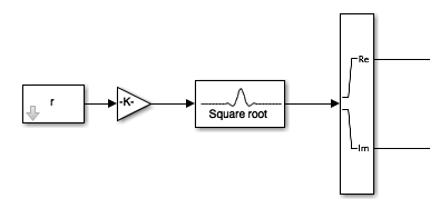
9. In prepration for Part 2, we will do something fancy to create a more computationally efficient design.
   
   
   1. Modify the portion of your Simulink design before the CCW Rotation block to look like this:
      
      
   
   
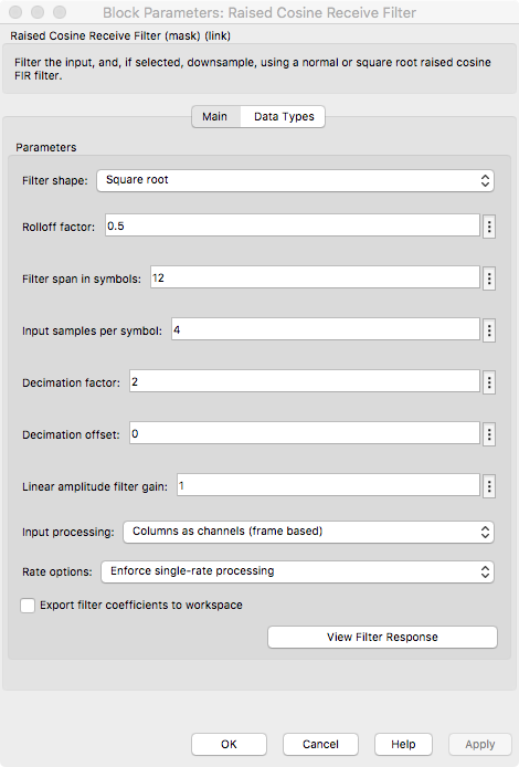
   2. The "Square Root" block is
      
      Communications System Toolbox -> Comm Filters -> Raised Cosine Receive Filter
      
      This block performs the same matched-filter-and-downsample operations as your earlier design, but performs this operation in a more computationally efficient manner using a polyphase filterbank (See Section 9.3 of the text).
   
   
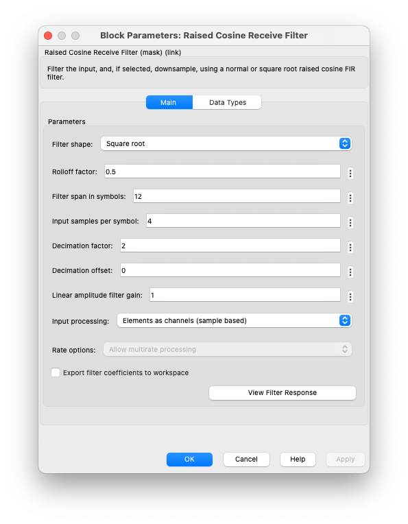
   3. Double-click on the "Square Root" block to open the Block Parameters Dialog Box. Set the block parameters as follows:
   
   
   4. Run the simulation.
   
   
   5. Confirm the system works the same as the previous system.

Part 2

Set Up the Pluto Radio Interface

1. Replace the Signal From Workspace block with system shown below
   
   
   
   
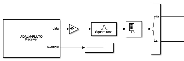
2. The ADALM-PLUTO Receiver block is located at
   
   Communications System Toolbox Support Packages -> ADALM-Pluto Radio Receiver
   
   Double click on the box to open the parameter dialogue box. Set the parameters as shown below:
   
   
   
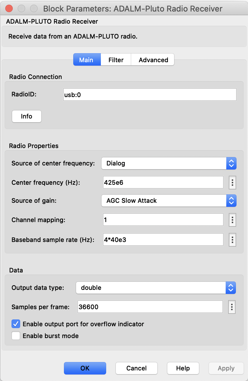
   Note that the baseband sample rate (BasebandSampleRate parameter) is set to 4 samples/symbol. If you change this, you will have to change the downsample rate in the matched filter.
   
   The Pluto Radio outputs a "frame" of data each time Simulink "calls" the interface function. This is done to help boost real-time performance. Each function "call" to the Pluto Radio requires a great deal of networking overhead. If, for example, each "call" to the Pluto Radio requested a single sample, the networking overhead would be applied to each sample, and the achievable sample rate would be embarrassingly low. Here, each "call" to the Pluto Radio produces 36600 samples (Simulink calls this a "frame") so that the networking overhead is amortized over the entire frame.
   
   
3. Because the Pluto Radio outputs a "frame" of data at a time, we need to alter the settings in the matched filter block. Double click on the block to open the properties dialogue and set the block parameters as follows:
   
   
   
   
   1. The number of samples per symbol and the "decimation factor" (I call it downsample factor) are a function of the input sample rate as described above. The settings shown here assume a sample rate equivalent to 4 samples/symbol from the Pluto radio.
      
      
   2. The input processing is set to "Columns as channels (frame based)" to maximize efficiency. One could unframe the data at the Pluto radio output and use sample-based processing here. But, because the data is already framed, the system runs faster the way it is shown.
      
      
   3. Single rate processing is enforced here because frame-based processing is used. The downsample by 2 simply reduces the size of the frame by a factor of 2.
   
   
   
4. The "Unbuffer" block is located at
   
   DSP System Toolbox -> Signal Management -> Buffers -> Unbuffer
   
   The "Unbuffer" block converts frames to a serial stream of samples. This is required at this point because the PLLs are recursive. Following MATLAB's recommendation for best practices, we have waited as long as possible before converting from frame-based processing to sample-based processing.
   
   
5. Note that in the second step, the OverflowOutputPort box was checked. Checking this box enables the second output from the Pluto Radio Receiver block called "overflow." An "overflow" occurs when the Pluto Radio is ready to output a new frame, but the Simulink model is not ready to process it. That is, the Simulink system falls behind and the data collected by the Pluto Radio is lost. Connect the Display block, located at
   
   Simulink -> Sinks -> Display
   
   This allows you to monitor the performance of your Simulink system.

Connect the Pluto Radio

1. Connect the Pluto Radio to your computer using the USB cable accompanying the Pluto radio.
   
   
2. At the Matlab prompt, type
   
   

   >> plutoradiosetup();
   				

Exercise

1. Set the Model Configuration Parameters as follows:
   

   Simulation time
   Start Time:	0.0
   Stop Time:	5
   Solver options
   Type:	Fixed-step
   Solver:	discrete (no continuous states)




2. Run the simulation.



3. Your demodulator runs for 5 seconds, which corresponds to 200,000 symbols. If properly designed, your PLLs have plenty of time to lock and you should detect approximately 75 occurrences of the PRE field described above.



4. To find the data, look for the 64 bit (32 symbol) PRE pattern in the detector output. You should find it approximately 75 times. After each occurrence the following 5404 bit decisions (2702 symbol decisions) correspond to 772 7-bit ASCII characters. Determine the message using your Matlab script. Note there are two messages!



5. Notes:
   
   
   • Scopes and other displays require a lot of computing resources and can slow the speed at which your demodulator operates. Try to use as few scopes as possible.
   
   
   • The only "display" I used was the Constellation Diagram block.
   
   
   • In my design, I performed differential decoding in Simulink using look-up tables. But you may perform differential encoding in a Matlab script. Whichever approach you take, but sure to use the differentially decoded data to find the secret message(s).