The Phase Lock Loop (PLL)

Introduction

In this exercise, you will design a discrete-time PLL and explore the differences between a first-order PLL and a second order PLL.

A block diagram of a discrete-time PLL is shown below. When the loop filter is a constant, the resulting system is a first-order PLL. When the loop filter is a proportional-plus-integrator filter, the resulting system is a second-order PLL. In this exercise you will explore the behavior of both first-order and second-order PLLs.

You will find a series of questions below. Document your answers to these questions using your favorite word processing software. Print the answers to the questions and turn in the printed document before you leave.

Textbook References

Appendix C. This exercise is based on the first example in Section C.2.1.

Exercise

First Order PLL

In Simulink, construct the PLL above using blocks from the Simulink Toolbox.

For the PLL input, use two Sine Wave blocks, one configured to be a cosine and the other to be a sine, as inputs to the Real-Imag to Complex block. (Note this is similar to how a complex-valued PLL output is produced.)

Design the loop filter to create a first-order loop with a closed-loop equivalent noise bandwidth of 0.2% of the sample rate. The relationship between the loop filter constant and the closed-loop equivalent noise bandwidth is the solution to Exercise C.7 (c).

Attach one scope to the output of the phase error detector.

Attach another scope to the real part of the input and the real part of the DDS output. You want to plot both sinusoids on the same set of axes.

At the signal source, set the frequency of the source to 0.01 cycles/sample, set the initial phase to 90 degrees, and set the sample time to 1.

Set the frequency of the DDS to 0.01 cycles/sample.

Set the simulation parameters as follows:

Simulation Time
Start time: 0.0	Stop time: 1000
Solver selection
Type: Fixed-step	Solver: discrete (no continuous states)

Run the simulation.

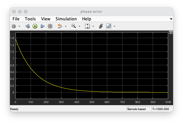
The phase error plot should look like this.

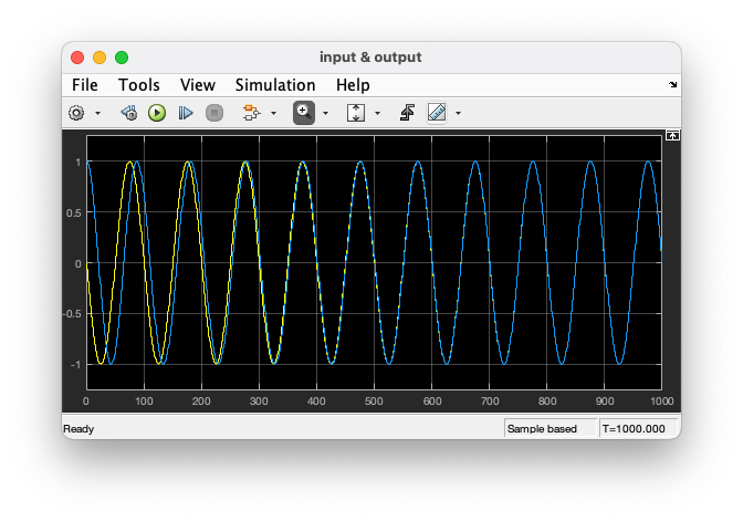
The input/output plot should look like this.
Answer the following questions.
- What is the relationship between the phase error and the two sinusoids?
- What is the significance of the initial phase error?
- How long did it take for the PLL to lock?
- What is the relationship between lock time and the closed loop bandwidth?

Change the initial phase of the source to 180 degrees.

Run the simulation.

Based on the phase error plot and input/output plot, answer the following questions.
- What is the relationship between the phase error and the two sinusoids?
- What is the significance of the initial phase error?
- How long did it take for the PLL to lock?
- What is the relationship between lock time and the closed loop bandwidth?

Change the frequency of the source to 0.0105 cycles/sample (but leave the DDS frequency unchanged).

Run the simulation with the stop time set to 2500.

Based on the phase error plot and input/output plot, answer the following questions.
- What is the relationship between the phase error and the two sinusoids?
- What is the significance of the initial phase error?
- How long did it take for the PLL to lock?
- What is the relationship between lock time and the closed loop bandwidth?
- How do your observations compare with the first row in Table C.1.1?

Second-Order PLL

In Simulink, construct the PLL above using blocks from the Simulink Toolbox.

Design the loop filter to create a second-order loop with a closed-loop equivalent noise bandwidth equal to 0.2% of the sample rate and a damping constant of 0.7071. [The relationship between the loop filter constants and the closed-loop equivalent noise bandwidth and damping constant are given by (C.58).]

Set the parameters of the signal source as follows: frequency = 0.0105 cycles/sample, initial phase = 180 degrees, sample time = 1. (These are the settings after step 14 in the previous section.)

Make sure the DDS frequency is 0.01 cycles/sample.

Use the same Simulation Configuration Parameters as before, except set the simulation stop time to 2500.

Run the simulation.

Based on the phase error plot and input/output plot, answer the following questions.
- What is the relationship between the phase error and the two sinusoids?
- What is the significance of the initial phase error?
- How long did it take for the PLL to lock?
- What is the relationship between lock time and the closed loop bandwidth?
- How do your observations compare with the third row in Table C.1.1?
- Compare the shape of the phase error curve obtained here with the shape of the phase error curve from step 15 above. Is the relationship between the two what you expected?