Symbol Timing Synchronization for BPSK

Introduction

The previous BPSK Simulink Exercise assumed the phase of carrier and the bit clock were known. That is, you knew the phase of the unmodulated carrier and you knew where the symbols began and ended. Unfortunately, this is not the case in practice -- in a real system the detector knows neither the carrier phase nor the bit (or symbol timing). The bit (or symbol) timing information must be extracted from the received samples. This is accomplished using a bit (or symbol) timing synchronizer. In this exercise, you are given the carrier phase (i.e., it is known), but in contrast, the bit (or symbol) timing is not known.

In this exercise, you will design a bit timing synchronizer for BPSK based on the PLL. There are three sample rates in play in this design, so you must be careful in assigning sample times to the Simulink blocks. The detector, with its accompanying bit timing synchronizer, will be used to process the modulated sampled in the file bpsktrdata.mat.

Textbook References

M-ary QAM: Section 5.3, discrete-time realizations: Section 5.3.2, partial response pulse shapes: Section A.2, general discussion of timing synchronization:, discrete-time techniques for symbol timing synchronization for binary PAM: Section 8.4, discrete-time techniques for symbol timing synchronization for BPSK: Section 8.5.

Specifications

normalized sample rate: 8 samples/bit normalized carrier frequency: 0.3 cycles/sample carrier phase 0 degrees average energy: 1 pulse shape: SRRC (50% excess bandwidth, span = 12 symbols) bit clock offset: unknown!! input file bpsktrdata.mat packet format: TR = 1000 bits (you don't need to know what they are) SYNC = 1 0 1 0 1 0 1 0 0 1 0 1 0 1 0 1 DATA = 3808 bits (544 7-bit ASCII characters)

Preliminary Design

Design the Detector

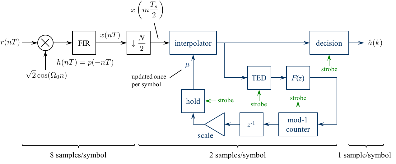
Design the detector, shown below, using blocks from the Simulink, DSP System, and Communications System Toolboxes.



Design the loop filter to create a second order loop to the following specifications: closed-loop equivalent noise bandwidth = 0.01 (normalized to the bit rate), damping factor = 0.7071.

Design Notes

1. Because the early-late TED operates at 2 samples/symbol, the matched filter output (at 8 samples/symbol) is downsampled by 4.


2. Use a Farrow interpolator. You can use either the piecewise-parabolic version (Figure 8.4.17) or the cubic version (Figure 8.4.18).


3. For interpolation control, use the decrementing modulo-1 counter described in Section 8.4.3. Use the underflow condition in the decrementing mod-1 counter as the strobe. The strobe is used as an enable signal for the TED, decision, and mu update.


4. You need to create an "enabled" version of the early-late TED. When the strobe is asserted, the TED output is given by equation (8.34). When the strobe is not asserted, the TED output is zero.


5. For the fractional interval (mu) update, use an "enabled hold" block. The "enabled hold" block outputs the previous value when the strobe is not asserted, or passes the input to the output when the strobe is asserted. This block is needed because the fractional interval is updated by the mod-1 counter only once per symbol, but the interpolator operates at 2 samples/symbol. The hold operation ensures that the interpolator is using the proper value for the fractional interval.
   
   Simulink provides a skeletal enabled subsystem:
   
      Simulink -> Ports & Subsystems -> Enabled Subsystem
   
   The default enabled subsystem is shown below
   
   
   
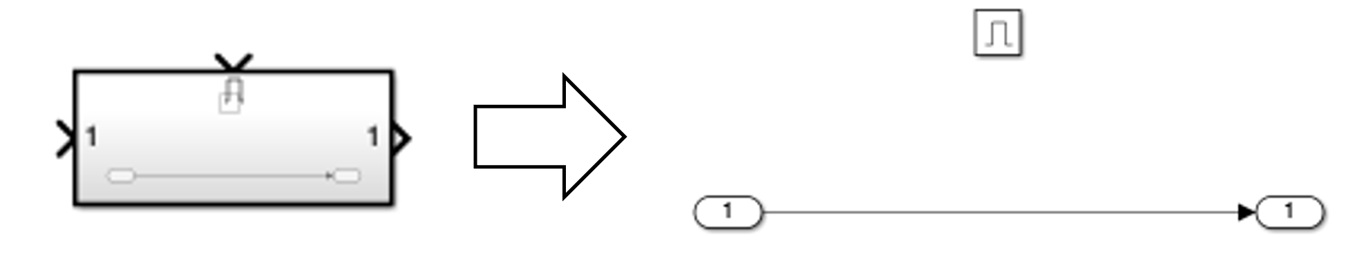
   The subsystem consists of a simple wire with the enable icon above it. This means the wire is only active when the enable signal is asserted. When the enable signal is not asserted, nothing happens and the output holds its value.


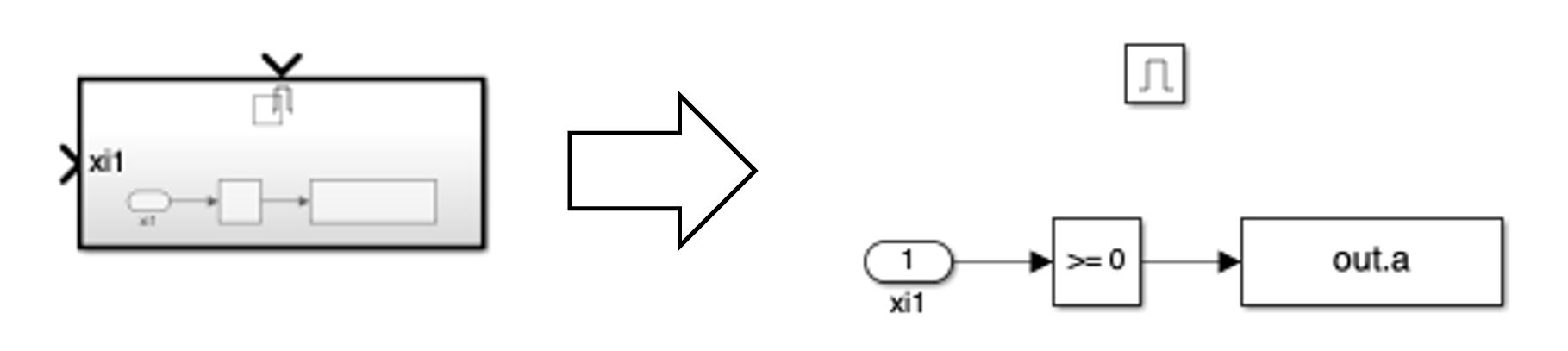
6. The decision subsystem is also enabled. This is because decisions should be made on every other interpolator output on average. The enable signal indicates which interpolator outputs represent the desired signal space projections. An example of the enabled decision subsystem for binary PAM is shown below
   
   

Exercise

1. Incorporate the symbol timing synchronization PLL into a BPSK detector.


2. For the detector input, use the From File block and set the Filename to bpsktrdata.mat and the sample time to 1.


3. Set the simulation parameters as follows:
   
   

   Simulation Time
   Start time: 0.0	Stop time: (12+1000+3808+2)*8
   Solver selection
   Type: Fixed-step	Solver: discrete (no continuous states)

   
   Note that the stop times is 2 bit times longer than the message. This is to allow the simulation to produce the last bit or two of the message because the input sample rate is approximately 8 samples/bit.


4. Run the simulation.


5. The detector produces approximately 4840 bit decisions. (The exact number depends on the number of times the strobe is high. This, in turn, depends on the dynamics of your symbol timing PLL.)


6. To find the data, look for the 16 bit SYNC pattern in the detector output. Once you find it, the following 3808 bit decisions correspond to 544 7-bit ASCII characters. Determine the message using either your Matlab script or an ASCII Table.


7. Plot the fractional interpolation interval (mu) and use this plot to estimate how long (measured in bits) it took for your timing PLL to lock.