M-ary Pulse Amplitude Modulation (PAM)

Introduction

In the previous exercise, the detector was for binary communications: each transmitted waveform is selected from a set of 2 possible waveforms and conveys one bit of information (since one bit is required to select one of two possibilities). Now we will consider M-ary communications where M is greater than 2. In this case there are M possible waveforms. Because log2(M) bits are required to select one of M possibilities, each waveform conveys log2(M) bits of information. Now each transmitted waveform represents a log2(M)-bit symbol.

This exercise builds on the already familiar baseband modulation by generalizing to the case of M = 8 symbols. This means each symbol represents log2(8) = 3 bits. Modulation is straightforward as well as most of the detection process. But look out, you'll have to generalize the functionality of the DECISION block to complete the assignment! All this will be used to process the secret message contained in the file bb8data.mat

Textbook References

PAM: Section 5.2, discrete-time realizations: Section 5.2.2, full response pulse shapes: Section A.1.

Specifications

normalized sample rate: 16 samples/symbol average energy 189 pulse shape: HS symbol clock offset: 0 input file bb8data.mat input message length: 140 symbols (420 bits or 60 ASCII characters)

Preliminary Design

Design the Detector

Design the detector, shown below, using blocks from the Simulink, DSP System, and Communications System Toolboxes.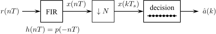

Design Notes

The only thing that is really new here is how the DECISION block works. Clearly, the decision is based on which constellation point is closest to the projection of r(nT) onto the signal space. There are several ways to do this, such as nested if statements comparing the projection of r(nT) with the decision boundaries, or fooling around with the magnitude and the sign of the projection of r(nT), etc. The most straightforward thing to do is to compute the squared Euclidean distance between the projection of r(nT) and all the points in the signal space and choose the index of smallest one as the output. You can use basic blocks from the Simulink block set to compute the squared Euclidean distance between the current projection and the M possible constellation points. To determine the index of the smallest, use the following block.

   DSP System Toolbox -> Statistics -> Minimum

When the parameter mode is set to index, this block returns the index of the minimum element in the input vector. The index is in the range [1,M] when the index base is set to One, or [0,M-1] when the index base is set to Zero.

Hint: To compute the Euclidean distance between each downsampled matched filter output and all M=8 constellation points, store the 8 constellation points in a row-vector using the Constant block:

   Simulink -> Sources -> Constant.

The difference between the downsampled matched filter output (a scalar) and the vector of constellation points is vector where each element in the vector is the difference the corresponding constellation point and the downsampled matched filter output. Subsequent operations involving this vector also produce vectors. Eventually, you should wind up with a vector of M squared Euclidean distances. This is the vector that forms the input to the Minimum block.

Test the Detector Design

Test the detector you designed by constructing a modulator to produce a test signal. The following procedure steps you through this design process:

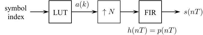
1. Design the modulator shown below to meet the above specifications except make the input the four symbol sequence 0 2 5 6.
   
   
   
   


2. Connect the output of your modulator to the input of your detector.


3. Connect the output of your detector to a To Workspace block (be sure to open the Properties Dialog Window and set the Save format to matrix) and a Scope block.


4. Set the simulation parameters as follows:
   
   

   Simulation Time
   Start time: 0.0	Stop time: 4*16
   Solver selection
   Type: Fixed-step	Solver: discrete (no continuous states)



5. Run the simulation and plot the demodulator input and the matched filter output on the same set of axes. Check the values in the workspace to see if they agree with input sequence 0 2 5 6.


6. Observe the values output by the Downsample block. Adjust the "Sample offset" of the Downsample block to obtain the proper values.

Exercise

1. Replace the modulator blocks with the From File block and set the Filename to bb8data.mat and the sample time to 1.


2. Set the simulation parameters as follows:
   
   

   Simulation Time
   Start time: 0.0	Stop time: 16*140
   Solver selection
   Type: Fixed-step	Solver: discrete (no continuous states)



3. Run the simulation.


4. The detector produces approximately 141 symbol estimates. The last 140 of these correspond to 60 7-bit ASCII characters. Determine the message using either your Matlab script or an ASCII Table.


5. Plot the eye diagram and signal space projections.