Binary Pulse Amplitude Modulation (PAM)

Introduction

In this exercise, you will design a binary baseband detector to process the noisy modulated data contained in the file bb2data.mat.

Textbook References

PAM: Section 5.2, discrete-time realizations: Section 5.2.2, full response pulse shapes: Section A.1.

Specifications

normalized sample rate: 16 samples/bit average energy 1 pulse shape: NRZ symbol clock offset: 0 input file bb2data.mat input message length: 126 bits (or 18 ASCII characters)

Preliminary Design

The goal of this Simulink exercise is to design and construct a detector. To test the detector, you need to design and construct a modulator. The following procedure steps you through this design process.

Create a New Simulink Model for Your Design

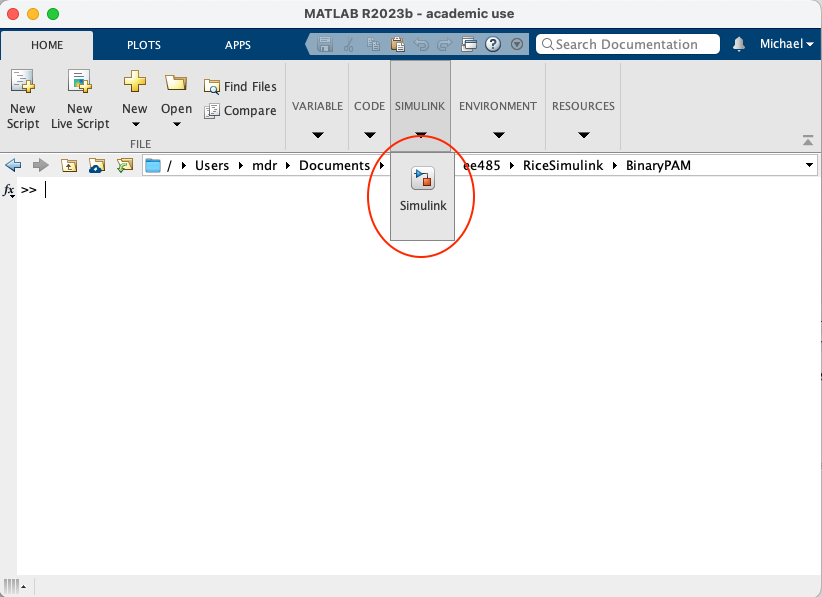
1. Start Matlab.


2. Select the Simulink tab along the top as shown below and select Simulink.
   
   
   
   
3. This opens the Simulink window shown below.
   
   
   
   
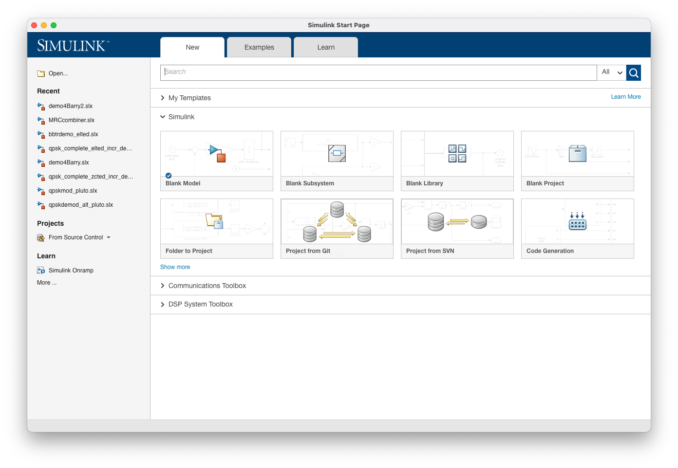
4. Select Blank Model. This opens the Simulink design window shown below.
   
   
   
   
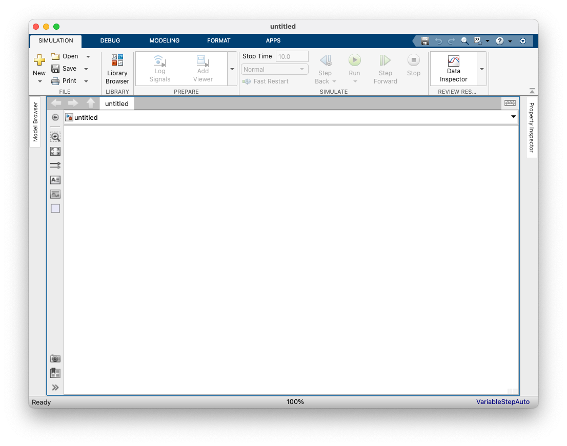
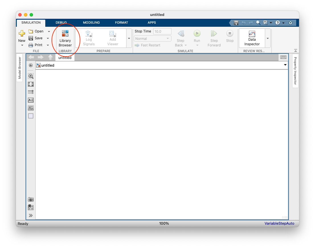
5. To access the blocks required to design the modulator and detector, open the Library Browser. Select the Library Browser shown below.
   
   
   
   
6. The Library Browser opens to the left of the Simulink design window as shown below.
   
   
   
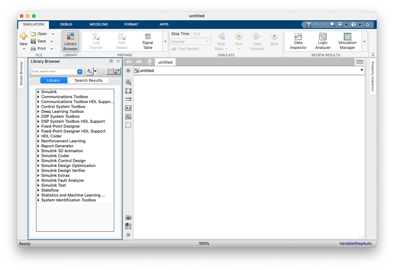
   Each item a triangle is pointing to is a toolbox in the Simulink Library. Your Simulink Library may have more toolboxes or fewer toolboxes. The toolboxes you will be using for this class are the
   • Simulink Toolbox
   • Communications Toolbox
   • DSP System Toolbox

Design a Modulator to Test the Detector Design

1. Design a modulator to test the detector. A block diagram of the modulator is shown below.
   
   
   
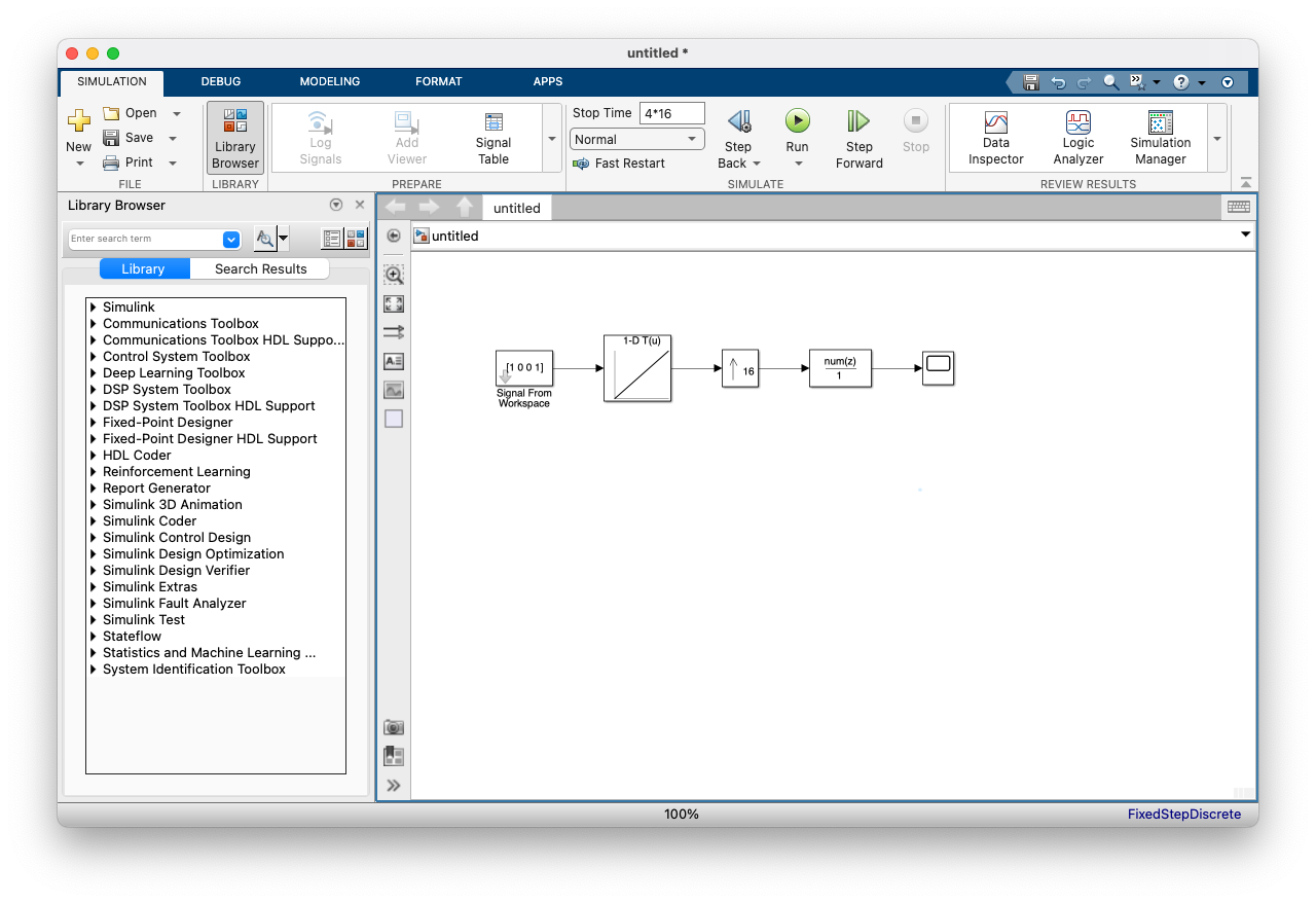
   The Simulink version of the modulator is shown below. Design the Simulink modulator to meet the above specifications except make the input the four-bit sequence 1 0 0 1.
   
   
   
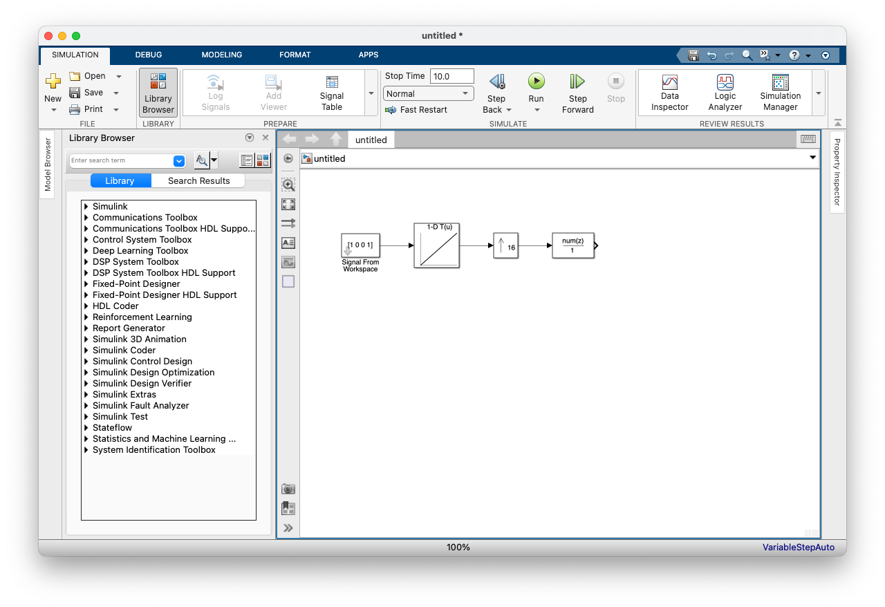
   This modulator comprises four blocks. These blocks, their locations, and their settings are described as follows.
   
   
   1. The first block is the Signal From Workspace block:
      
         DSP System Toolbox -> Sources -> Signal From Workspace
      
      Drag this block to your design window. Double-click the Signal From Workspace block to open Block Parameters Dialog box. Set the block parameters as illustrated below.
      
      
      
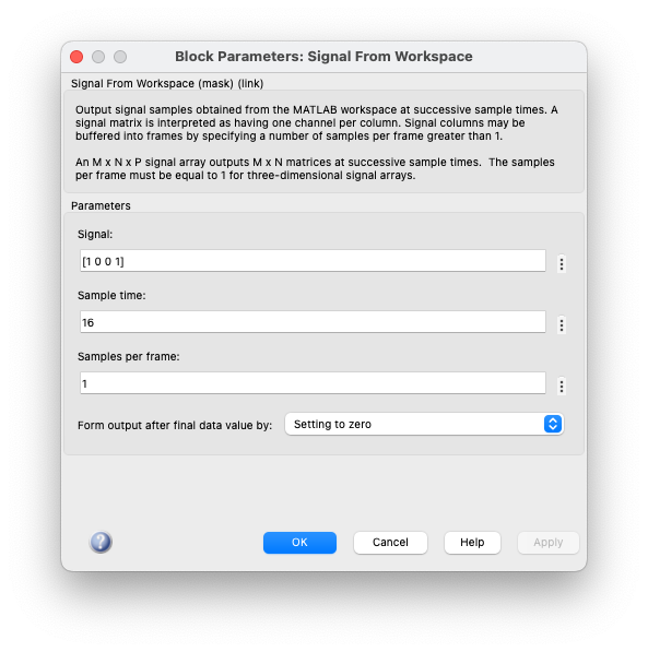
      The first parameter is a column vector defining the input data. The second parameter specifies the sample time. We want to normalize all sample times to the sample rate. Because there are N=16 samples/bit, 16 is entered in this field. Because will will not be doing any frame buffering in this exercise, leave the third parameter alone. The last parameter specifies what to do when the end of the workspace vector is reached but the simulation is still running. The options are to append zeros, repeat the last value, or cycle back to the beginning of the workspace vector. It will not matter what you choose for this simulation: you can leave it at the default setting as shown.
   
   
   2. The second block is the Look-up Table block:
      
         Simulink -> Lookup Tables -> 1-D Look-Up Table
      
      Drag this block to your design window. Double click the Look-Up Table block to open Block Parameters Dialog box. Set the block parameters as shown below.
      
      
      
      "Table data" is the vector contining the constellation points. "Breakpoints 1" is a vector containing the bit values.
   
   
   3. The third block is the Upsample block:
      
         DSP System Toolbox -> Signal Operations -> Upsample
      
      Drag this block to your design window. Double click the Upsample block to open Block Parameters Dialog box. Set the block parameters as shown below.
      
      
      
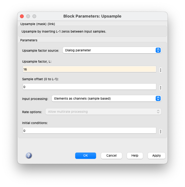
      The "Upsampled factor, L" is the upsample factor which is the number of samples/bit. The "Sample offset" specifies the number of zeros produced before the first input sample. This should be zero for the modulator. Set "Input processing" as shown.
   
   
   4. The fourth block is the Discrete Filter block:
      
         Simulink -> Discrete -> Discrete Filter
      
      The filter block is used to perform pulse shaping. Drag this block to your design window. Double click the Discrete Filter block to open Block Parameters Dialog box. Set the block parameters as shown below.
      
      
      
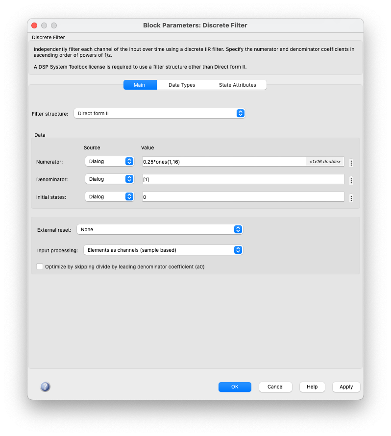
      Be sure to set "Input processing" as shown.


2. Test the modulator by completing the following:
   
   
   1. Connect a scope (Simulink -> Sinks -> Scope) to the output of the pulse shaping filter as shown below.
      
      
      
      
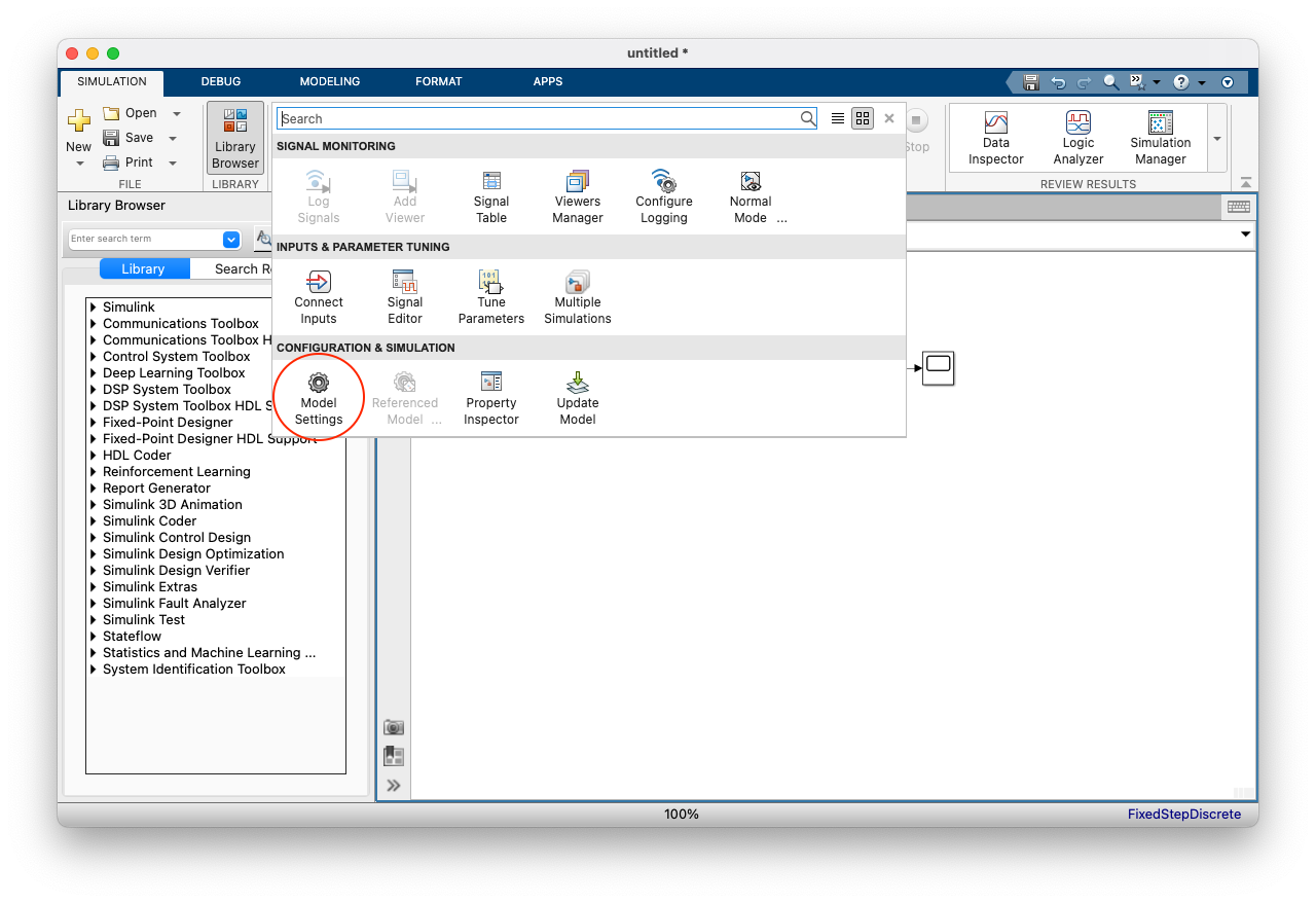
   2. In preparation for running the model, the Model Configuration Parameters must be set properly. To do this, click the down arrow shown in the image below.
      
      
      
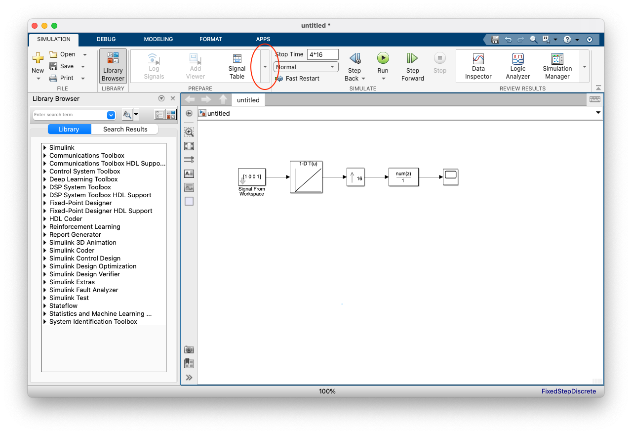
      Select Model Settings as shown below.
      
      
      
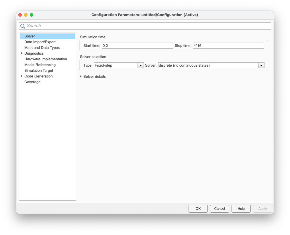
      This opens the Configuration Parameters dialog window shown below. Set the Simulation time and Solver selection parameters as shown below.
      
      
      
      
   
   
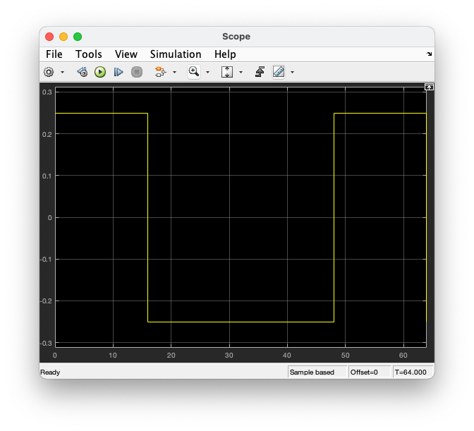
   3. Run the simulation by selecting the green "Run" button at the top of the Simulink model window.
   
   
   4. The result should be a plot as shown below. (You may have to double-click the scope block in the Simulink model to open the Scope window.)
      
      

Design and Test the Detector

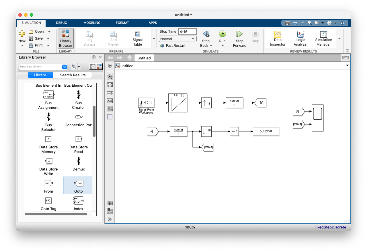
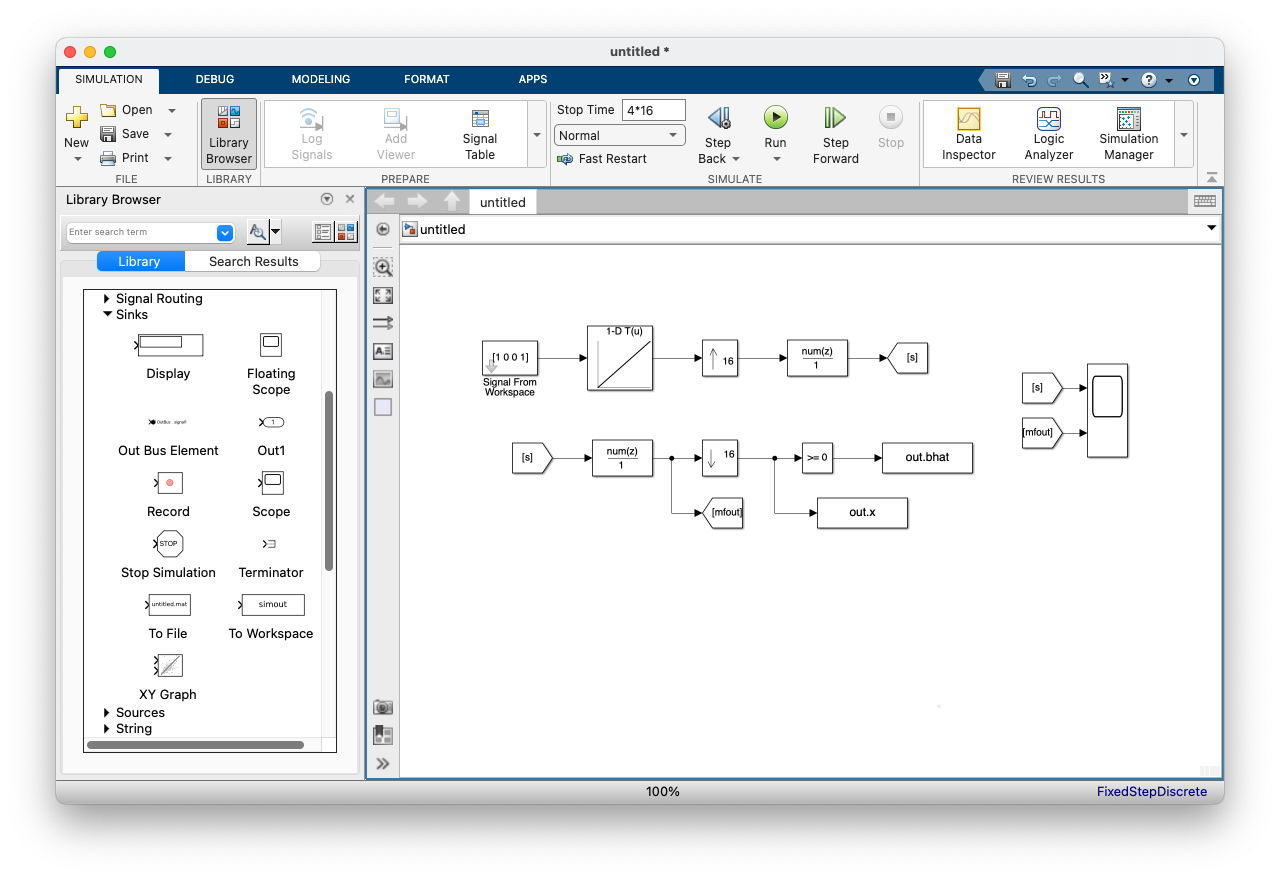
1. Design the detector, shown below, using blocks from the Simulink, DSP System, and Communications System Toolboxes.
   
   
   
   
2. Connect the output of your modulator to the input of your detector.


3. Connect the output of your detector to a To Workspace block. The result should look something like the image below.
   
   
   
   Notes:
   
   
   • The matched filter uses the same Discrete Filter block used for the pulse shaping filter.
   
   
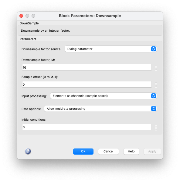
   • To downsample the matched filter output, use the Downsample block:
     
        DSP System Toolbox -> Signal Operations -> Downsample
     
     Drag this block into your design window. Double-click the Downsample block to open the Block Parameters dialog box. Set the block parameters as shown below.
     
     
     
     
   • The decision block is a compare-to-zero operation performed by the Compare To Zero block:
     
        Simulink -> Logic and Bit Operations -> Compare To Zero
     
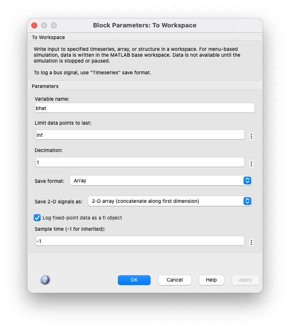
     Drag this block into your design window. Double-click the Compare To Zero block to open the Block Parameters dialog box. Set the Operator to ">=".
   
   
   • The bit decisions should be sent to the Matlab workspace. To accomplish this, use the To Workspace block:
     
        Simulink -> Sinks -> To Workspace
     
     Drag this block into your design window. Double click the To Workspace block to open the Block Parameters dialog box. Set the block parameters as shown below.
     
     
     
     


4. Keeping the same simulation Configuration Parameters used to test the modulator, run the simulation. The plot of the transmitted signal and the matched filter output should look the plot below.
   
   
   
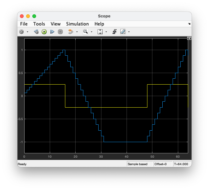
   The solid yellow line is the received signal (the test signal) and the blue line is the matched filter output. As you can see, the first valid bit decision occurs at sample 16 which corresponds to the first peak observed in the matched filter output. The three subsequent bit decisions at samples 32, 48, and 64 correspond to the next three bits in the data sequence. If you look in the workspace, you will notice that the detector output 5 decisions instead of 4. This is because the Downsample block output an initial 1 at sample 0. Does the workspace variable agree with the input sequence (1 0 0 1)?


5. Determine if the downsampling instant (bit timing synchronization) is correct. To determine this, attach the output of the Downsample< another To Workspace block as shown below.
   
   
   
   Run the simulation. For this exercise, the value of "x" should be
   
      0 1 -1 -1 1
   
   You will observe that it is not. This is because the Downsample block is keeping the wrong samples. To correct this, change the "Sample offset" property of the Downsample block so that the right matched filter output sample is kept. Once you have worked out the proper downsample offset, you are ready to do the Simulink exercise.


6. Plot the signal space projections. Use the Constellation Diagram block:
   
      Communication Toolbox -> Comm Sinks -> Constellation Diagram
   
   Connect the input to the Constellation Diagram block to the output of the downsample block. Double click on the Constellation Diagram block. This opens a plot Simulink plot window. To modify the settings to work with this lab, complete the following:
   
   
   1. Click the PLOT tab at the top of the plot window.
   
   
   2. Click Settings (with the gear icon).
   
   
   3. Set the DATA AND AXES fields as follows:
      

      Number of input ports	1
      Samples per symbol	1	Offset	0
      Symbols to display	200
      X limits	[-2, 2]	Y limits	[-1, 1]
      Bring to front	grayed out
      check Grid	check Color fading

      
      
   4. Click the X in the upper right corner to close the dialog.
   
   
   5. Click the PLOT tab at the top of the plot window.
   
   
   6. Click Reference Constellation
   
   
   7. Set the Reference Constellation fields as follows:
      

      check	Show reference constellation
      Input	1
      Reference Constellation	BPSK
      Average reference power	1
      Reference phase offset (rad)	0

   
   
   8. Click Apply.
   
   
   9. Click the X in the upper right corner to close the dialog window.

Exercise

1. Replace the modulator blocks with the From File block:
   
      Simulink -> Sources -> From File
   
   Double-click the From File block to open the Block Parameters Dialog box. Set the File name to bb2data.mat and the sample time to 1.


2. Set the simulation parameters as follows:
   
   

   Simulation Time
   Start time: 0.0	Stop time: 16*(18*7)
   Solver selection
   Type: Fixed-step	Solver: discrete (no continuous states)



3. Run the simulation.


4. The last 126 bits of the detector output represent 18 ASCII characters. Determine the message using either your Matlab script or an ASCII Table.


5. Plot the signal space projections.